Using Monte Carlo simulation for financial forecasting
 Metals are some of the most widely used and mature commodities in the world. Despite their ubiquitous nature and sophisticated engineering methods, the financial modelling tools used by most miners remain simplistic. Deregulation of energy markets in the latter part of the 20th century brought with it a wave of new and innovative products designed to both better understand and increase the value of energy assets. Some of these techniques have been adopted by other industries, but less so by metals and mining companies. This appears to be partly because of the complexities of simultaneously modelling multiple revenue and cost items. One way to perform this type of analysis is by using Monte Carlo analysis, which can be used to solve problems when multiple variables may make calculating an answer difficult or impossible, and when the answer can be expressed in terms of probability of occurrence. While there is dedicated software available to perform this type of analysis, it has not been widely adopted, and is not necessary.
Discussing new concepts and ideas is a worthwhile exercise, but without real answers to real problems, concepts and ideas tend to remain just interesting topics of conversation. This article will describe one way to set up a Monte Carlo analysis to be used by a mining company to answer two seemingly simple questions. Before describing the proposed solution, we will discuss some of the challenges of selecting model inputs, and take the reader through two examples which demonstrate the importance of correlation and volatility on mining companies. In the online version of this story, we will provide instructions on how to set up a Monte Carlo simulation tool capable of answering the questions posed in the in the Case Study example.
Case Study
Hypothetical Mining Company (HMC) has monthly production of 176,000 oz. of silver, 2,300 oz. of gold, 1,000 MT of zinc, and 150 MT of copper, and consumes 7,000 bbl of diesel per month (that works out to 1 bbl per oz. of gold equivalent production). HMC has monthly revenue of US$10.3 million based on current market prices of US$16.30 per oz. silver, US$1,300 per oz. gold, US$3,475 per tonne zinc, and US$6,900 per tonne copper. At US$80/bbl diesel, HMC has a monthly diesel expense of US$560,000. Like a lot of mines, HMC has operated sporadically over the years, coming into production when prices were high and going on care-and-maintenance when prices were low. When operating, the mine has a stable production profile and, aside from diesel expense which varies monthly, the mine’s other costs are stable at US$9 million per month.
After speaking to the mine manager, the CFO has asked, “We need to make some equipment investment decisions. What’s the chance the mine will be unprofitable one year from now?”
Upon returning from a meeting with the head of investor relations, the CFO asks, “We have been telling investors we are a silver company. I am concerned the run-up in zinc prices is making us look like a zinc company. How certain can we be silver is going to contribute more than 25% of our monthly revenue in two years?”
These questions are much more complex than they may sound. There is no formula we can just plug numbers in and get answers out. One way to answer these questions is by using Monte Carlo analysis.
It’s worth taking a moment to consider what the answers might look like. This is a step that should probably be done more often. Conceptualizing the answer is important when building spreadsheets and other tools which can get overly complex. Questions that start with, “What’s the chance…” and “How certain can we be…” can be answered with distributions of possible outcomes. Both questions have an element of time to them and the solution needs to simultaneously display probability distributions at different time horizons.
The answer to the first question is: There is a 35% chance the mine will be unprofitable in 12 months (based on our model inputs). The chart below (Fig. 1) is based on the results of Monte Carlo analysis. Read the chart as saying that with n probability the margin will be below the line corresponding to the month you are looking at. There is a 35% chance the margin will be below zero in 12 months, a 95% chance the margin will be less than $3.3 million, and a 5% chance the mine will lose $1.8 million.
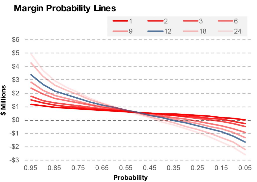
Figure 1
The answer to the second question is: There is approximately a 28% chance silver will be contributing less than 25% of the total monthly revenue in two years. The chart below (Fig. 2) is another example of an output from Monte Carlo analysis. The x-axis is the number of simulations run. You can see that after only a thousand simulations the “answer” is still quite volatile, but as more data points are added the line becomes more stable at the estimated value. (this chart is included as an example for this problem. the number of runs (data points) should be explicitly evaluated prior to analysis. some question may require only a few hundred runs while other questions may require many many more than even the 4,000 we use here.)
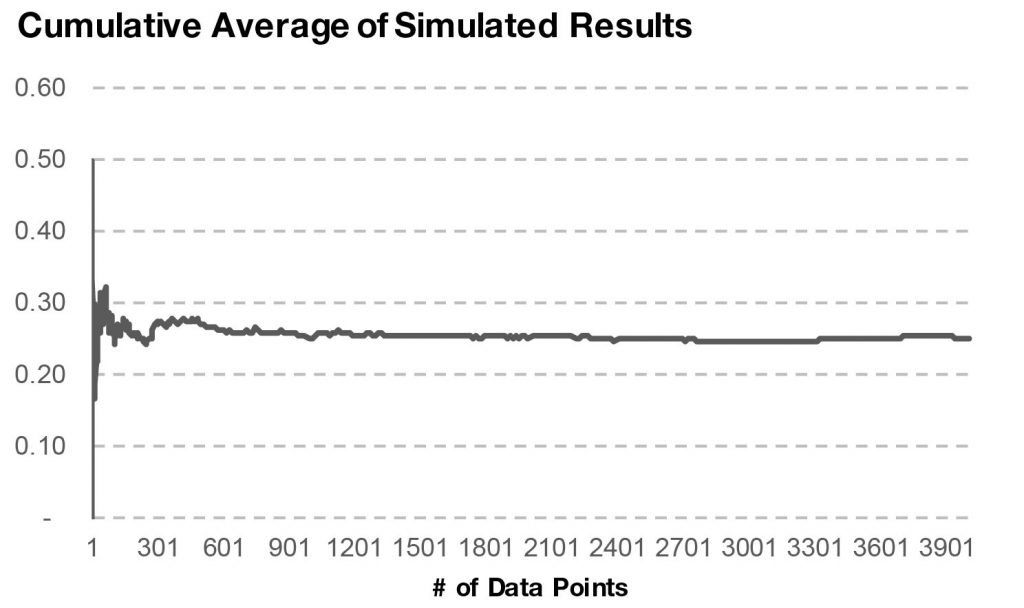
Figure 2
Importance of Model Inputs
It’s important to understand the quality of output depends very strongly on the quality of inputs. If we want to project future revenues, our production forecast and projections of prices, volatilities and correlations are required and must be of high quality.
Many companies rely on analyst forecasts, or the views of senior management for price forecasts. This approach has some flaws: analyst forecasts tend to change in response to what’s already happened in the markets; forecasts rarely offer a margin of error; and there’s a tendency to assign more credibility to bullish forecasts and discount the advice of bearish forecasts. Explaining prices which differ significantly from observable market forward prices may pose other challenges. One possible solution is to use market based forward/futures prices, although one needs to be aware that forward prices do not always reflect the most likely spot prices in the future, and that factors such as liquidity can influence their usefulness.
Similar challenges exist in projections of volatilities. We will rely on at-the-money implied volatilities from the option markets as inputs for our tool to demonstrate the model set-up. It needs to be understood that these are only useful approximations that might be misleading at times.
Finally, the biggest challenge in building reliable projections of future revenues is finding proper input correlations; this topic is quite complex. The simplest approximation would involve estimating either return correlations on historical forward prices, or correlation on historical spot prices. To achieve decent quality, the estimation would require significant analysis. For our purposes, just as we are using observable prices and volatilities from the financial markets, we will use a recent 60-month correlation of monthly average prices as the correlation inputs to answer the two questions.
We need to underscore that this general prescription is just a starting point and projecting production volumes, prices, and especially volatilities and correlations, requires careful consideration.
The impacts of correlation and volatilities on mining companies
Most mining companies produce more than one metal which contributes to revenues, and most also have some variable costs such as energy and foreign exchange. The interaction between variable revenue and cost items can impact financial results. Understanding the potential financial impacts of these interactions is important.
To put in perspective the importance of correlation on mining, let’s consider just the interaction of gold and diesel prices since 2000.
A representative gold producer uses 1 bbl of diesel for every ounce of gold produced and has an average AISC of US$1,100 per oz. Today gold is selling for US$1,300 per oz. and diesel can be purchased for US$80/bbl (so AISC ex-Oil is US$1,100 – US$80 = US$1,020 per oz.) and current margin is US$200 per oz.
Diesel costs 6.2% of the price of gold (US$80 per bbl / US$1,300 per oz.). In percentage terms, since 2000, the price of diesel has been as much as 21% of the price of gold, and as little as 3% of the price of gold. Fig. 3 is a chart of diesel prices expressed as a % of the price of gold since 2000.
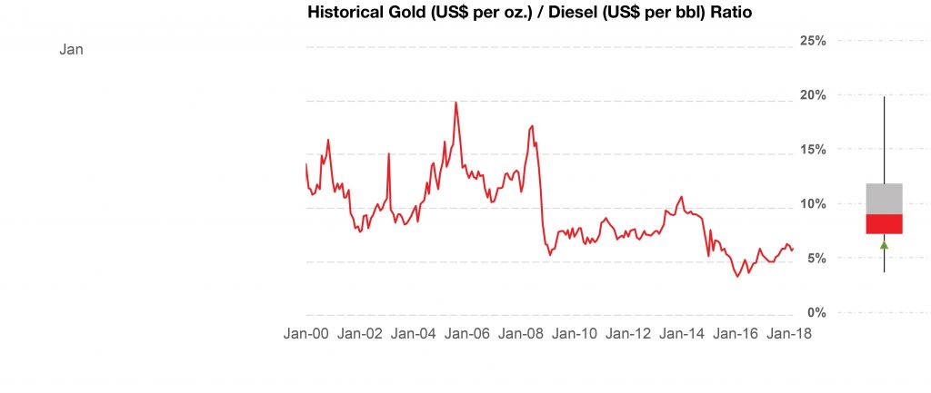
Figure 3
Now, let’s look at the impact an increase in diesel price as a percentage of the price of gold has on the margin of a producer with an AISC ex-oil of US$1,020/oz. If we think about diesel being US$80/bbl and gold being $1,300/oz, it might be easy to convince ourselves that US$80 is small, and the variability of that US$80 is even smaller, so it’s not worth worrying about. This is clearly not the case when considering the potential impact on margins, and you can see that in the charts below.
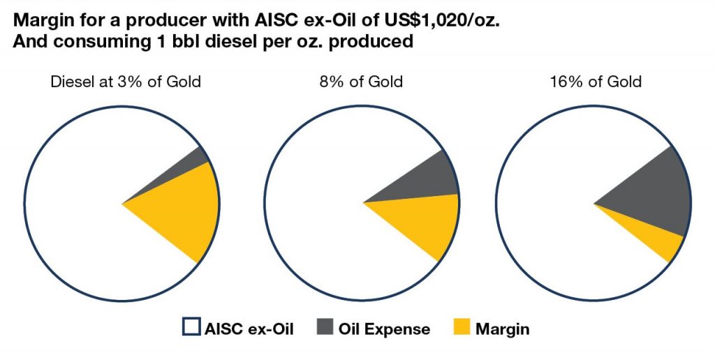
Figure 4
For the gold producer with an AISC ex-Oil of US$1,020 per oz., the impact of the interaction of oil and gold prices has the potential to wipe out margin. However, if the AISC-ex Oil was US$800per oz. the impact of diesel prices in absolute terms would be the same, but the reduction in margins in percentage terms would be less, and arguably not worth worrying about. Fig. 5 is a chart of the percentage change in margin as a function of changes in diesel prices relative to gold prices for a producer with an AISC of US$800 per oz. and one with an AISC ex-Oil of US$1,020 per oz.
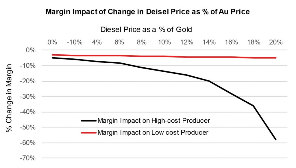
Figure 5
Experience shows us high-cost miners run their businesses very similarly to low-cost miners despite the fact that decreasing margin increases sensitivity to correlation and volatility. Remember, margins can decrease because of a reduction in selling prices, but increased costs such as labour contracts and royalty agreements can decrease margin and result in increased sensitivity to correlation and volatility. These effects should be carefully considered during the evaluation process. Factors such as correlation and volatility are more important to high-cost mines than low-cost mines.
Let’s look at an example using HMC (Hypothetical Mining Company) with monthly production of 176,000 oz. of silver, 2,300 oz of gold, 1,000 MT of zinc, and 150 MT of copper. Currently, HMC has revenue of $10.3 million per month split 30% each from silver, gold and zinc and 10% copper. If we assume the production profile has been constant and look at just the impact of prices on revenues for the past 10 years, we see the mine has had monthly revenues of as little as US$5.05 million (October 2008) and as much as US$15.7 million (April 2011). In that same time, silver contributed from 25% to 54% of revenue, gold 16% to 36%, zinc 15% to 48% and copper 7% to 15%. Sometimes HMC has been a silver company, sometimes a gold company, and sometimes a zinc company.
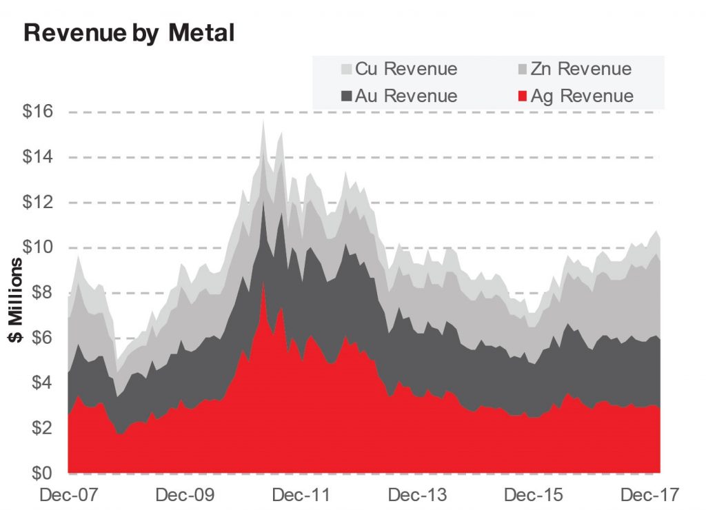
Figure 6
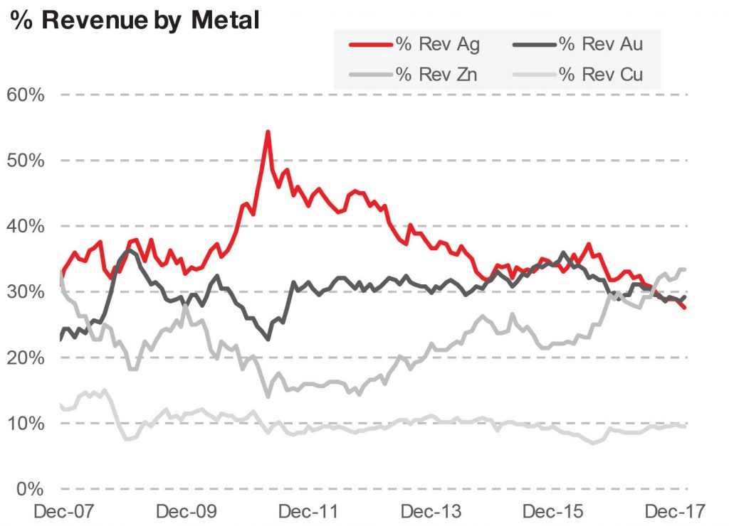
Figure 7
One thing has been constant, correlation (or lack of correlation) and volatility of prices has been as important to HMC’s story as it has been to the company’s financial health and forecast.
The two examples above highlight important challenges for mining companies. In the first example, the variability of oil with respect to gold prices had the potential to wipe out margins, and this will show up in AISC. In the second example, the mine’s monthly revenue has been in a range of US$5 to US$15 million and the dominant source of revenue has shifted and forced the company to “pick and choose” which one is the primary metal and which are accounted for as byproducts. Perhaps even more important are the challenges these interactions create when compiling financial forecasts.
Price interactions such as the ones described above are complex, but well suited for Monte Carlo analysis. Model inputs require careful consideration beyond what we have discussed. Remember, what matters today may not matter tomorrow and what doesn’t matter today may be important tomorrow. A lack of understanding of correlation and volatility, along with outdated financial modelling techniques, has the potential to erode investor confidence in management’s descriptions of the past and predictions for the future.
Now, we’ll go step-by-step through the set-up of a spreadsheet for modelling up to five random correlated variables, providing a viable framework for the answering the questions posed in the Case Study.
Detailed instructions for setting up a tool in Excel
Below we describe in detail the Excel set-up of a Monte Carlo simulation. Array functions, named ranges and macros could greatly simplify the workbook, but will not be used. Only formulas which can be keyed directly into the formula bar of Excel will be used. This will make the result accessible to all readers regardless of Excel proficiency. The result will be a less elegant spreadsheet, but an equally powerful Monte-Carlo simulation tool capable of modeling up to five variables. By building the spreadsheet from scratch you will gain valuable insight into the problem and the solution, and it will seem like less of a black-box.
Once you have built the spreadsheet you can see for yourself how expectations change with changes in prices, volatilities, correlations, costs, or production forecasts. More sophisticated Excel users can use this tool to estimate the value of simple and complex options, assess the effectiveness of risk-management decisions, and add value by allowing better-informed investment decisions with a dynamic, objective, and quantitative method for assessing the business.
Let’s get back to answering our questions by first restating them.
After speaking to the Mine Manager, the CFO has asked, “We need to make some equipment investment decisions. What’s the chance the mine will be unprofitable 1 year from now?”
Upon returning from a meeting with the Head of Investor Relations, the CFO asks, “We have been telling investors we are a silver company. I am concerned the run-up in zinc prices is making us look like a zinc company. What’s the probability silver is going to contribute less than 25% to our monthly revenue in two years?”
Open a new Excel workbook and start in cell B3. Red numbers and letters are row and column references and do not need to be input.
In cells B3:C11 should key in the following, this is the production profile for HMC.
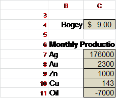
Bogey is the costs after oil for HMC. Notice Oil is a cost and so is entered as a negative number. Later, if you want to replace production with costs use a negative number.
In cells E5:L11 put in the following table of information

The top row is the number of months forward from now.
Now moving to volatilities set up a new table to the right of the prices.

As with the price table, this is a table of at-the-money implied volatilities for the forward tenors. In cell N6 you can input the formula =E6 and drag that to column U6 and that will show the months forward if that helps you keep track, but it isn’t necessary.
Our last set of user specified inputs will be correlations.

The shading in the cells is meant as a visual guide that these are he cells you should change if you want to refresh the data.
It’s important that you have input the tables in the same rows and columns. It may be tempting right now to start including your own data but try to curb your enthusiasm so you can make sure the sheet is working correctly before including your own data.
In cell B21 put in the text “Cholesky Matrix”. We will put formulas in cells C22:G26 so that our final-result looks like this:

Now we will list the formulas you should input into each cell.
C22 =SQRT(C15)
C23 =C16/$C$22
C24 =C17/$C$22
C25 =C18/$C$22
C26 =C19/$C$22
Let’s move to column D
D22 can be left empty
D23 =SQRT(1-C23^2)
D24 =(D17-C24*C23)/D23
D25 =(D18-C25*C23)/D23
D26 =(D19-C26*C23)/D23
Column E
E22 empty
E23 empty
E24 =SQRT(E17-(C24^2+D24^2))
E25 =(E18-(C25*C24+D25*D24))/E24
E26 =(E19-(C26*C24+D26*D24))/E24
Column F
F22 empty
F23 empty
F24 empty
F25 =SQRT(F18-(C25^2+D25^2+E25^2))
F26 =(F19-(C26*C25+D26*D25+E25*E26))/F25
Column G
G22 empty
G23 empty
G24 empty
G25 empty
G26 =SQRT(G19-(C26^2+D26^2+E26^2+F26^2))
If you have input the same values for the User Specified Correlations and the formulas correctly, you should have the same values in your sheet as in the Cholesky Matrix table above. These values will change if you change the User Specified Correlations.
The Cholesky Matrix is really the hardest part. The entire rest of the workbook only requires about as many formulas as we just input.
Let’s quickly put in some text headers to help us see what’s left and to keep track of what we are working on.
In Row 39 put the following text into these cells
B39 = Normal Random Variables
H39 = Correlated Random Variables
O39 = Inferred Forward Ag Prices
X39 =Inferred Forward Au Prices
AG39 =Inferred Forward Zn Prices
AP39 =Inferred Forward Cu Prices
AY39 =Inferred Forward Oil Prices
BH39 = Inferred Future Revenue Less Bogey
BQ39 =Chance Zinc is < 25% of Revenue
Now a few more text notes
N40 =Months Fwd
N41 =% of a Year
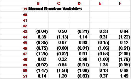
Now we are going to create normal random variables. In cell B43 input the following formula
B43 =NORMINV(RAND(),0,1)
Now, drag that formula across to column F and down to row 4042.
This is generating random numbers with mean of 0 and standard deviation of 1. Your numbers will not be the same as these, but your cells A39:F4042 should look similar to this:

If you hit the F9 key the numbers will change.
Now, we are going to use those Random Variables and the Cholesky Matrix from above to generate Correlated Random Variables also with mean of 0 and standard deviation of 1.
Starting in cell H43, we will input formulas in H43:L43 and I will list them below
H43 =B43
I43 =B43*$C$23+C43*$D$23
J43 =B43*$C$24+C43*$D$24+D43*$E$24
K43 =B43*$C$25+C43*$D$25+D43*$E$25+E43*$F$25
L43 =B43*$C$26+C43*$D$26+D43*$E$26+E43*$F$26+F43*$G$26
Highlight cells G43:L43 and drag those formulas down to row 4042.
Notice in column H you should have the same values as in column B, but in columns I, J, K, and L you should have new random numbers. These new random numbers have mean of 0, standard deviation of 1, and are correlated as you specified in the User Specified Correlation Matrix. Hitting the F9 key will change the numbers.
It’s time to start generating some Inferred Forward Prices.
Put these formulas in cells O40 and O41
O40 =E6
O41 =O40/12
Drag these formulas over to column V so you should have the following:

This step makes the next set of formulas easier to write and follow by displaying the number of months forward we specified earlier, and converting them to % of a year in row 41.
Let’s populate the inferred forward prices
O43 =E$7*EXP((-N$7*N$7/2)*O$41+N$7*SQRT(O$41)*$H43)
And drag that across to column V and down to row 4042
X43 =E$8*EXP((-N$8*N$8/2)*O$41+N$8*SQRT(O$41)*$I43)
And drag that across to column AE and down to row 4042
AG43 =E$9*EXP((-N$9*N$9/2)*O$41+N$9*SQRT(O$41)*$J43)
And drag that across to column AN and down to row 4042
AP43 =E$10*EXP((-N$10*N$10/2)*O$41+N$10*SQRT(O$41)*$K43)
And drag that across to column AW and down to row 4042
AY43 =E$11*EXP((-N$11*N$11/2)*O$41+N$11*SQRT(O$41)*$L43)
And drag that across to column BF and down to row 4042
Now we are going to deduct the $9 million Bogey from the inferred future revenue for each time column and express the result in US$ millions.
BH43 =($C$7*O43+$C$8*X43+$C$9*AG43+$C$10*AP43+$C$11*AY43)/1000000-$C$4
And drag that across to column BO and down to row 4042
All that’s left now is to answer the questions the Mine Manager and the Head of Investor Relations asked. To answer the Mine Manager
In cell Q16
Q16 =E6
And drag that formula across to column X
P17 =.95
P18 =.90
And so-on down to P35 = .05
Now, in cell Q17
Q17 =PERCENTILE(BH$43:BH$4042,$P17) and drag that across to column X and down to row 35 so you should have a table similar to the following:
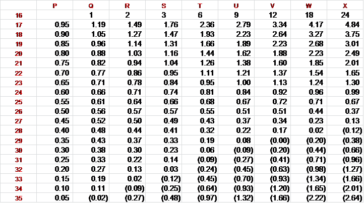
The answer to the first question, “What’s the chance the mine will be unprofitable a year from now?” can be found by going to the column for month 12 (column V in this case) and then working our way down to the first negative number which is at .35 and means there is a 35% chance the mine will be unprofitable in 12 months.
If you click any of the cells in the table and then in the menu at the top use Insert, and choose a line-chart you should get a chart similar to the one from earlier that fits neatly in the middle of the screen.
The answer to the second question requires a little bit of intuition.
In cell BQ42 put the following formula:
BQ43 =IF(($C$7*V43)/($C$7*V43+$C$8*AE43+$C$9*AN43+$C$10*AW43)<$BQ$40,1,0)
Now drag that formula down to row 4042. Then, in cell BQ40
BQ40 =.25
You can change BQ40 to test different % revenues coming from silver.
The answer is then found by taking the average of BQ by putting this formula in cell BQ41
BQ41 =AVERAGE(BQ43:BQ4042)
What we did here was, for each line divide the silver revenue by the total revenue, and if that is less than our test number we return a value of 1 and if not then return 0. By taking the average of these we get the probability silver will be less than our test value of the total revenue. In this case we see there is about a 20% chance silver will contribute less than 25% of total revenue in two years. If you hit F9 repeatedly you will notice that average bounces around from about .19 to .21 and we could correct that by adding more lines.
For interest, if you set BS43 =AVERAGE($BQ$43:BQ43) and then drag that down to row 4042 you will get the cumulative average of column BQ. Now, if you click on cell BS43 and again hit Insert and then line chart you can graph the cumulative average. Click F9 a few times and see how the average of the first few hundred data points is variable, but by the time you get to the right side of the chart the line become pretty stable at around 19% to 20%. This is a good illustration that the error in only a few observations is high but decreases as more data points are added.
How did we do it(?) and a quick note on one of the limitations
We generated random numbers in Excel with mean of 0 and standard deviation of 1 and then used a Cholesky decomposition to generate random correlated variables also with mean of 0 and standard deviation of 1. These random correlated variables were then converted to future possible prices using the Black-Scholes formula. The answer was then found by summarizing the data after generating enough paths so that the summarized data converged at the answer.
One limitation of the tool is that the convergence of the estimate might require more than 4,000 paths. Depending on the specific question we want answered and the collection of inputs, the proper answer might require many more paths. The questions we posed only required an estimate which we answered in 5% increments. Monte Carlo simulation as a technique is capable of answering much more sophisticated questions at much higher resolutions, but then the quality of inputs becomes critical, and the number of paths should be evaluated so that the possible margin of error in the result is well understood.
Chris Olmstead has 10 years of experience in investment banking and has also worked for Sempra Energy Trading, Alcoa, AK Steel, and UPS in a variety of structuring, risk management and procurement roles spanning metals and energy. Chris has a B.S. from Georgia Institute of Technology, an MBA from Ohio State University and is currently pursuing a Masters in Mining Engineering through South Dakota School of Mines and Technology.
Krzysztof Wolyniec is managing partner of Millwright Capital, a quantitative commodity fund. Previously, he was managing director of Commodity Quantitative Strategies at Sempra Energy Trading and Royal Bank of Scotland. He started his career at Mirant Corp., where he served as director of research. He has published widely on quantitative techniques in commodities and he is coauthor of “Energy and Power Risk Management” published by Wiley.
Comments